Simulation Examples

Now that you've read through all the simulation guides, let's bring it all together with a few quick examples. These examples will compare block diagrams with their qdex simulation equivalencies.

Example 1

This example uses two types of block connections, a gain element, and a transfer function to modify a sine wave. The result is output to a plot. In the equivalent qdex module, the simulation is started when the page is active (that is, open) and is stopped when the page is inactive.

<sectionNoTitle name="example1Section">

  <timePlot name="sinePlot" />
  
  <simulation name="simpleSim">
    <onActivePageChanged>
      if active then
        simpleSim:Start()
      else
        simpleSim:Stop()
      end
    </onActivePageChanged>
    <solver>
      <series>
        <sine amplitude="30" frequency="0.5" />
        <parallel>
          <gain value="3" />
          <transferFunction num="1 5" den="1 0 10" />
        </parallel>
        <probe ref="example1Section.sinePlot" />
      </series>
    </solver>
  </simulation>
  
</sectionNoTitle>

Example 2

This example uses multiple input signals, a feedback loop, and a number of math elements. The resulting waves are muxed together so that they can both be output to the same plot.

In the equivalent qdex module, the simulation is started when the user presses the button, and stops after 10 seconds. Note that to output both waves to the same plot, the series attribute in the timePlot declaration must be set to 2.

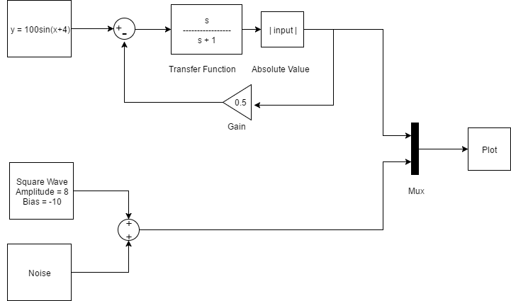
<sectionNoTitle name="example2Section">

  <timePlot name="thisPlot" series="2" />

  <button content="Start Simulation">
    <onClick>
      anotherSim:Start()
    </onClick>
  </button>

  <simulation name="anotherSim" duration="10">
    <solver>
      <series>
        <mux>
          <series>
            <sine amplitude="100" phase="4" />
            <feedback>
              <series>
                <transferFunction num="1" den="1 1" />
                <math op="abs" />
              </series>
              <gain value="0.5" />
            </feedback>
          </series>
          <sum>
            <square amplitude="8" bias="-10" />
            <signalGenerator waveform="random" />
          </sum>
        </mux>
        <probe ref="example2Section.thisPlot" />
      </series>
    </solver>
  </simulation>

</sectionNoTitle>

Example 3

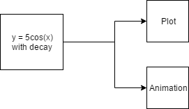
This is an example of a simple system being used to animate a shape. The source is created using a sine wave multiplied with a function in a system to create decay. Two plots inside a stack are used to plot the response and animate a ball.

<include src="plotTools.xml" />

<section name="animationSection">
  <title>Bouncy Ball</title>

  <stack name="plotStack" orientation="horizontal">
    <timePlot name="responsePlot">
      <axis dim="x" min="0" max="5" />
    </timePlot>
    <xyPlot name="ballPlot">
      <axis dim="x" auto="growAndShrink" major="false" />
      <axis dim="y" auto="lockAspectRatio" major="false" />
      <series name="path" draw="lineSegments" />
      <series name="ball" draw="radialFill" />
      <!-- Transparent frame used to steady the plot as the ball moves -->
      <series name="frame">
        <style>
          <foreground color="transparent" />
        </style>
        <data>-1 6; 6 6; 6 -1; -1 -1</data>
      </series>
    </xyPlot>
  </stack>
  
  <!-- Drawing the ball -->
  <script>
    plotTools.drawCircle(plotStack.ballPlot.ball, {0,5}, 0.1)
  </script>

  <button content="Start">
    <onClick>
      ballSimulation:Start()
    </onClick>
  </button>

  <simulation name="ballSimulation" duration="5" period="0.005">
    <solver>
      <series>
        <sine amplitude="5" phase="1.57" />
        <system>
          <input name="sineIn" width="1" />
          <output name="decaySine" width="1" />
          <onOutputs>
            -- Creating decay
            return vector({sineIn[1]*(1/(0.75*time+1))})
          </onOutputs>
        </system>
        <math op="abs" /> <!-- Faking the presence of the ground, making ball "bounce" -->
        <probe ref="animationSection.plotStack.responsePlot" />
        <probe ref="animationSection.plotStack.ballPlot.path" />
        <system name="drawBall">
          <input name="ballLocation" width="1" />
          <onOutputs>
            -- Translating the ball using the value of the response 
            plotStack.ballPlot.ball.Transform = matrixf.translation(time, ballLocation[1]-5, 0)
          </onOutputs>
        </system>
      </series>
    </solver>
  </simulation>

</section>