Attributes

To start a simulation, the first step is to create a new simulation element.

<simulation duration="10" period="0.1" asynchronous="false">
</simulation>

The simulation element has several attributes that determine its behaviour:

  • asynchronous is a flag that determines if the simulation should be run at a deterministic rate (synchronized to the timebase), or as quickly as possible. The default is false.
  • duration specifies the duration of the full simulation in seconds. The default is for an infinite duration (-1).
  • period is the period of the simulation loop in seconds. For example, a simulation that updates at 50Hz would have a period of 0.02s. We recommend not running simulations at rates faster than 100Hz or a period of 0.01s. The default is 0.01s.
  • loop is a flag that determines if the simulation should loop after it has reached its duration. The default is false.

Methods

Simulations have four methods that can be used to control their state.

  1. Start - Starts the simulation at time zero
  2. Stop - Stops the simulation and re-initializes its blocks
  3. Pause - Pauses the execution of the simulation
  4. Play - Resumes the simulation from current time after pausing

Theses methods are called from script, and can be called from a simulation event (e.g. onActivePageChanged) or from a control (e.g. a button).

<simulation name="firstSim">
  <onActivePageChanged>
    if active then
      firstSim:Start()
    else
      firstSim:Stop()
    end
  </onActivePageChanged>
</simulation>

<button name="myButton" content="Pause Simulation">
  <onClick>
    if myButton.Text == "Pause Simulation" then
      firstSim:Pause()
      myButton.Text = "Resume Simulation"
    else
      firstSim:Play()
      myButton.Text = "Pause Simulation"
    end
  </onClick>
</button>

Events

You can also declare a script that you want to run in response to the events that are triggered by simulations. The events that are available are:

  1.  onStateChanged - occurs when the simulation starts/stops or is paused/resumed
  2. onUpdate - triggered after each simulation loop is executed
  3. onDuration - triggered when the simulation is completed
  4. onActivePageChanged - occurs when the page is loaded on a device
  5. onDocumentOpened - occurs when the document is loaded on a device

Example

Using the onUpdate event to create a custom script for a simulation with a specified period is a good way to create a deterministic simulation that does not involve a traditional block diagram. For example, if you wanted to update the position of a falling rock for a simple physics simulation you could easily create a simulation and script that solves for the position of the rock at each time step. 

<label name="fall_distance">Distance fallen = 0 m</label>
<label name="elapsed_time">Time Elapsed = 0 s</label>
    
<button name="sim_button" content="Start">
    <onClick>
        if sim_button.Text == "Start" then
            sim_button.Text = "Stop";
            sim:Start();
        else
            sim_button.Text = "Start";
            sim:Stop();
        end
    </onClick>
</button>

<simulation duration="10" name="sim" period="0.01">
    <onUpdate>
       local distance = 0.5 * 9.81 * time^2;
       fall_distance.Text = string.format("Distance fallen = %.2f m", distance);
       elapsed_time.Text = string.format("Time Elapsed = %.2f s", time);
    </onUpdate>
    <onDuration>
       sim_button.Text = "Start";
    </onDuration>
</simulation>

When the button is pressed, the simulation runs for 10 seconds, updating the distance fallen by the rock every 0.01 seconds. The values are stored in a label at each time step. Note that time is the current simulation time and can be accessed inside of the onUpdate event. For information on inherent event variables, see the Scripting Reference.

The OutputsAt(int port) and OutputAt(int port, int signal) methods are also inherent methods that are members of simulation elements, and can be called in a script to access the current values at those locations in the model diagram.

Solvers

To create more complex simulations involving transfer functions or state-space models, you first have to define a solver. Solvers have the same general attributes as simulations themselves, including asynchronousperiod, and onUpdate. The period of a solver is the same as the simulation parent by default, though other periods can be specified as long as they are a multiple of the simulation rate. Multiple solvers can even be added to a single simulation with different periods to create parallel multi-rate simulations. Solvers include a general attribute which simulations do not have which is type. By changing the type of solver you are changing the numerical approach that your simulation will take to solve your model. Currently you can select between three solvers, which include:

  1. ode1 - Euler method
  2. ode2 - Heun's method
  3. ode4 - Runge-Kutta method    

The below examples demonstrate how to alter the simulation solver.

Example 1

<simulation period="0.01" duration="10">
  <!--Declaring type of solver-->
  <solver type="ode1">
    <series>
      <sine amplitude="0.1" frequency="3.57" />
      <transferFunction num="1" den="0.001867 0.000060498 1" />
      <probe ref="myPlot.mySeries" />
    </series>
  </solver>
</simulation>
ode1-sim.png

Example 2

<simulation period="0.01" duration="10">
  <!--Declaring type of solver-->
  <solver type="ode4">
    <series>
      <sine amplitude="0.1" frequency="3.57" />
      <transferFunction num="1" den="0.001867 0.000060498 1" />
      <probe ref="myPlot.mySeries" />
    </series>
  </solver>
</simulation>
ode4-sim.png

Connecting Blocks

When you initially create a simulation and define blocks, they are not connected together but independent elements in the simulation space. In order to connect the blocks and form your virtual block diagram, you need to define how the blocks are interconnected. There are several approaches that can be taken to wiring the blocks together.

Series

When blocks are placed into a series element, they are connected together in the order in which they are added to the block. For example, the following diagram shows how the elements in the following example would be connected:

series-blocks.jpg
<series>
    <transferFunction name="system1" num="1" den="1"/>
    <transferFunction name="system2" num="1" den="1"/>
    <transferFunction name="system3" num="1" den="1"/>
</series>

Parallel

The parallel elements behave in much the same way as the series elements, splitting a value between different paths, before combining them using a summation. The systems that are applied to the paths are connected in the order in which the elements appear in the parent. For example, to connect the same transferFunction elements in the earlier example you would change the series tags to parallel tags.

<parallel
    <transferFunction name="system1" num="1" den="1"/>
    <transferFunction name="system2" num="1" den="1"/>
    <transferFunction name="system3" num="1" den="1"/>
</parallel>
parallel-blocks.jpg

By default elements in parallel are added together. Elements can be subtracted or added by adjusting the polarity property, which indicates the polarity of each element being summed. The "+" symbol denotes positive polarity while the "-" symbol denotes negative polarity.

<parallel polarity="+--">
    <transferFunction name="system1" num="1" den="1"/>
    <transferFunction name="system2" num="1" den="1"/>
    <transferFunction name="system3" num="1" den="1"/>
</parallel>

Stack

The stack parental element can be used in a similar way to the parallel structure, but to separate values in parallel without the final summation block. For example, when combined with the demux and mux operators covered later in this guide, you can create systems that apply separate gains to separate elements in a vector like this:

<demux outputs="3"/>
<stack>
   <gain value="1"/>
   <gain value="2"/>
   <gain value="3"/>
</stack>
<mux inputs="3"/>

which translates into the following diagram

stack-blocks.jpg

Feedback

The feedback parent element is the final automated wiring option. The two elements that are placed into feedback blocks are treated as the open (or forward) loop element, and the feedback element in a closed-loop system. If only one element is provided, then it is treated as a closed-loop system with unity feedback. Feedback is negative by default. Take a look at the following code.

<feedback positive="true">
  <!-- Forward path -->
  <series>
      <!-- Controller -->
      <parallel>
          <gain name="Kp" value="20" />
          <series>
              <gain name="Kd" value="0.5" />
              <transferFunction name="derivative" num="1 0" den="1 100" />
          </series>
      </parallel>
      <!-- Plant -->
      <transferFunction name="plant" num="1" den="1 3 1" />
  </series>
</feedback>

Which creates the system below.

positive-feedback.jpg

Wire

The wire tool is a simple additional connection tool. When you create a wire element, you provide the signal that you want to form the connection from, and the connection that you want to to go to. The ports are formatted as follows:

<wire from="mySolver.mySystem.myPort.mySignal" ... />

If the signal is omitted, then the whole port is connected. If the port is left out, then the first port is connected. The system must be defined, but the solver also be left out as long as the connection is not made between multiple solvers. To connect ports to multiple destinations, a list of ports can be provided.

Source Blocks

Let's begin by discussing the sources that are available:

clock: The clock element is a source that outputs the current simulation time in seconds.

<constant name="scalar_const" value="5"/>
<constant name="vector_const" value="1 2 3"/>

constant: Can be used to define a scalar or vector constant.


<sine amplitude="5"/>

sine: Creates a sine wave. Can specify amplitude, bias, frequency, and phase.


<square amplitude="3" frequency="0.5" />

square: Creates a square wave. Can specify amplitude, bias, frequency, and phase


<step initial="1" final="3" time="5" />

step: Creates a step function. Can specify initial value, final value, and time that step occurs.


<ramp amplitude="0.5" />

ramp: Creates a ramp function. Can specify amplitude and bias.


<triangle amplitude="3" /> 

triangle: Creates a triangle wave. Can specify amplitude, bias, frequency and phase. 


<sawtooth amplitude="5" frequency="0.25" />

sawtooth: Creates a sawtooth wave. Can specify amplitude, bias, frequency and phase. 


<signalGenerator waveform="random" />

signalGenerator: Creates a wave of the specified type. Can specify amplitude, bias, frequency and phase. Waveform should be specified.


MULTIPLE WAVES

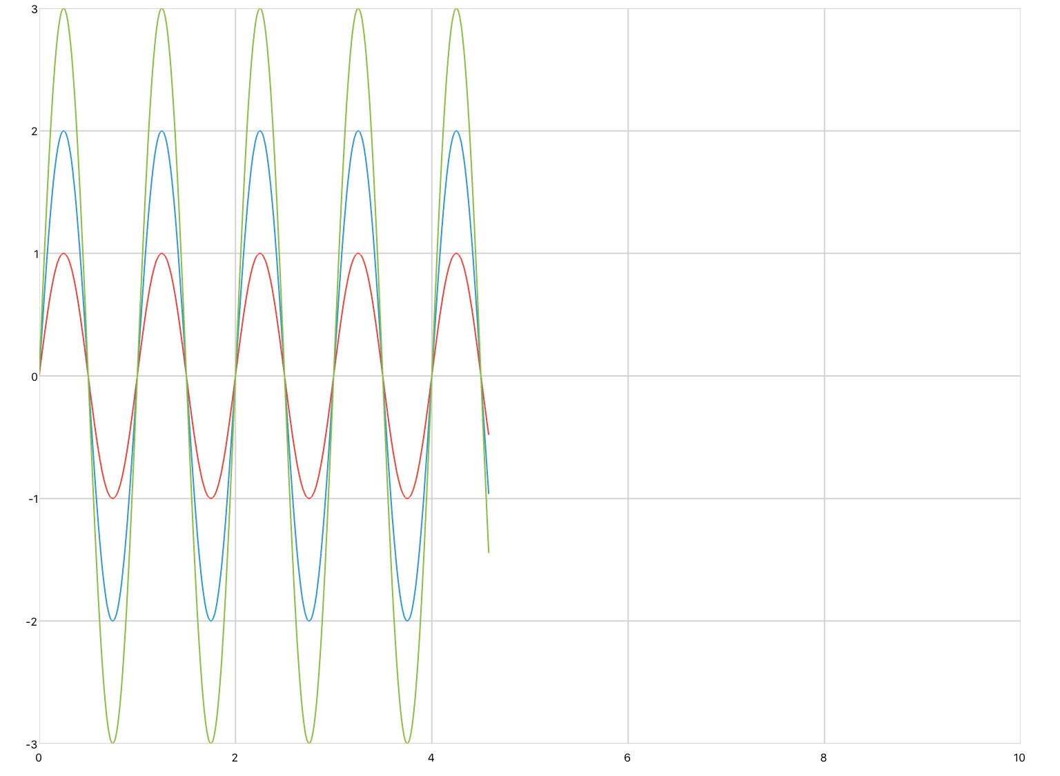
The waveform blocks can also be used to generate multiple waves in a vector without having to define the sources independently. The number of series in the plot must be specified.  

<timePlot name="myPlot" series="3" />

<simulation name="sineSim" duration="30" period="0.01">
  <solver name="solver">
    <series>
      <sine amplitude="1 2 3" />
      <probe ref="sectionName.myPlot" />
    </series>
  </solver>
</simulation>
 
multiple-source.jpg
 

Defining Your Model

Once you have added sources to your model, you will likely want to define a model using continuous systems. There are a few methods available to define a model.

Transfer Function

This element can be used to define a transfer function by entering the numerator and denominator. For example, the following code

<transferFunction num="23" den="0.13 1"/>

represents this system

 
transfer-function.jpg
 

A special feature of the transfer function blocks on the qdex platform is that they are designed to accept both scalar and vector inputs. This means that, for example, you could pass several datasets through a single transfer function representing a low-pass filter and it will apply the filter to all of them. This approach, along with similar approaches taken with several of the other blocks available using the framework, allows authors to create systems with fewer blocks than would be conventionally required.

State Space

This element is similar to the transfer function block, in that you can define an arbitrary model, but in this case as a state-space model of the form

 
state-space.jpg
 

The block contains attributes for the requisite ABC, and D matrices. These matrices are defined in a similar manner to the transfer function attributes, for example:

<stateSpace name="pendulum"
       a="0 0 1 0; 0 0 0 1; 0 149 -15 5; 0 -262 14 -8.6" 
       b="0; 0; 0; 0" 
       c="0 0 0 0; 0 0 0 0; 0 0 0 0; 0 0 0 0"
       d="0; 0; 0; 0"/>

creates a state space model that represents a rotary pendulum.

System

The system block can be used to create a completely custom system by first identifying the number of states, and then the input and output widths. Finally, you can define the value(s) that are used by the solver to calculate the derivatives and outputs of the system.

<system name="mycustom" states="1">
  <input name="u" width="1"/>
  <output name="y" width="1"/>
  <onDerivatives>
    return states + u[1];
  </onDerivatives>
  <onOutputs>
    return vector({3 * math.sin(2 * math.pi * time) + states[1] - u[1]});
  </onOutputs>
</system>

When the solver is called at each time-step of the simulation, it triggers the onDerivatives event, which is responsible for providing the value(s) that are used by the solver to calculate the derivative of the state(s). It also calls the onOutputs event which uses Lua script to calculate the output at each time step. In this manner, you can create arbitrary linear or non-linear system definition.

Data Output

Probe

The probe is used to pass data from a particular part of the simulation to a destination outside of the simulation. This can be used to update the values displayed in labels or tables, or passed to plots. In the following example the output from the plant is sent to a table in another part of the document:

<transferFunction name="plant" num="1" den="1 3 1" />
<probe ref="myDemo.mytable.outputRow.outputColumn.outputLabel"/>

and in this example the sine waves are sent to a plot to be rendered:

<simulation name="simulation" duration="10" period="0.02">
    <solver>
        <series>
            <mux>
                <sine amplitude="3" />
                <sine amplitude="2" />
                <sine amplitude="1" />
            </mux>
            <probe ref="myExperiment.myDrawing.theplot" />
        </series>
    </solver>
</simulation>

Typically when plotting simulation data you should use a timePlot, as it automatically plots the data against the simulation sample time. You can also output points to an xyPlot, where the data passed through the probe will be treated as X-Y pairs. To do this, simply set the time attribute on the probe to false.

The probe element also has a conditional attribute which will only write data when specified. When the conditional attribute is set to true, a second input port opens. When a non-zero value is passed through this second port the probe will write data to the referenced XML element. When a zero value is passed through the second port, no data will be written from the probe. In this example data is only written to the target when the simulation time is greater than 1 second.

<simulation name="mySim" period="0.01"> 
  <solver>
    <series>
      <system>
        <output name="out" width="6" />
        <output name="enable" width="1" />
        <onOutputs>
          <![CDATA[
          if time < 1 then
            enable = vector({1})
          else
            enable = vector({0})
          end
          return DataSend, enable
          ]]>
        </onOutputs>
      </system>
      <!--Only writing DataSend to target when enable is greater than zero-->
      <probe ref="mySection.CommStream" conditional="true" />
    </series>
  </solver>
</simulation>

Signal

The signal element is similar to the probe, but acts in the opposite direction. Creating a signal element allows you to access an external data source and integrate it into your simulation directly without the need for additional Lua scripting. For example, the following code would take the value from a slider and use it as an input to a feedback loop.

<slider name="myslider"/>
<simulation duration="10" name="sim" period="0.1">
    <solver>
        <series>
            <signal ref="mysection.myslider"/>
            <feedback>
              ...
            </feedback>
      </series>
  </solver>
</simulation>

This same method can be used to connect a button, text input, etc.

Math, Logic, Compare

There are several elements that can be defined in simulations to update signals using mathematical operations. These blocks are:

gain: Multiplies a scalar or vector signal by the value of the gain. Supports both element-wise and matrix multiplication, set using the mode attribute.

product: Finds the product of the inputs to the block, or any subsystems provided. Includes a reciprocality attribute to set the reciprocality of each element being multiplied (* or /).

divide: Computes the division of its two inputs.

sum: Finds the sum of the inputs specified. If only one input is provided, it finds the sum of the elements in a vector. 

subtract: Finds the difference between two inputs.

Math Block

There is also a math block, which performs common mathematical operations such as trigonometric and exponential functions. Set the operation using the op attribute when defining the block:

<math op="degToRad" />

The different operations that are available are:

abs
A unary operation which computes the absolute value of each element of the input signal.

acos
A unary operation which computes the inverse cosine of each element of the input signal.

acosh
A unary operation which computes the inverse hyperbolic cosine of each element of the input signal.

acot
A unary operation which computes the inverse cotangent of each element of the input signal.

acoth
A unary operation which computes the inverse hyperbolic cotangent of each element of the input signal.

acsc
A unary operation which computes the inverse cosecant of each element of the input signal.

acsch
A unary operation which computes the inverse hyperbolic cosecant of each element of the input signal.

asec
A unary operation which computes the inverse secant of each element of the input signal.

asech
A unary operation which computes the inverse hyperbolic secant of each element of the input signal.

asin
A unary operation which computes the inverse sine of each element of the input signal.

asinh
A unary operation which computes the inverse hyperbolic sine of each element of the input signal.

atan
A unary operation which computes the inverse tangent of each element of the input signal.

atan2
A binary operation which computes the arctangent of each element of the first input signal with the corresponding element of the second input signal. If either input is a scalar, then the scalar is applied for each element of the other signal.

atanh
A unary operation which computes the inverse hyperbolic tangent of each element of the input signal.

ceil
A unary operation which computes the ceiling of each element of the input signal.

cos
A unary operation which computes the cosine of each element of the input signal.

cosh
A unary operation which computes the hyperbolic cosine of each element of the input signal.

cot
A unary operation which computes the cotangent of each element of the input signal.

coth
A unary operation which computes the hyperbolic cotangent of each element of the input signal.

csc
A unary operation which computes the cosecant of each element of the input signal.

csch
A unary operation which computes the hyperbolic cosecant of each element of the input signal.

degToRad
Converts each element of the input signal from degrees to radians.

exp
A unary operation which computes the exponential of each element of the input signal.

floor
A unary operation which computes the floor of each element of the input signal.

ln
A unary operation which computes the natural logarithm of each element of the input signal.

log
A binary operation which computes the logarithm of each element of the first input signal using the corresponding element of the second input signal as the base. If either input is a scalar, then the scalar is applied for each element of the other signal.

log10
A unary operation which computes the base-10 logarithm of each element of the input signal.

log2
A unary operation which computes the base-2 logarithm of each element of the input signal.

mod
A binary operation which computes the modulus of each element of the first input signal with respect to the corresponding element of the second input signal. If either input is a scalar, then the scalar is applied for each element of the other signal.

pow
A binary operation which computes the power of each element of the first input signal to the corresponding element of the second input signal. If either input is a scalar, then the scalar is applied for each element of the other signal.

pow10
A unary operation which computes ten to the power of each element of the input signal.

pow2
A unary operation which computes two to the power of each element of the input signal.

radToDeg
Converts each element of the input signal from radians to degrees.

reciprocal
A unary operation which computes the reciprocal of each element of the input signal.

rem
A binary operation which computes the IEEE remainder of each element of the first input signal with respect to the corresponding element of the second input signal. If either input is a scalar, then the scalar is applied for each element of the other signal.

round
A unary operation which computes the rounded value of each element of the input signal.

sec
A unary operation which computes the secant of each element of the input signal.

sech
A unary operation which computes the hyperbolic secant of each element of the input signal.

sign
A unary operation which computes the sign of each element of the input signal.

sin
A unary operation which computes the sine of each element of the input signal.

sinh
A unary operation which computes the hyperbolic sine of each element of the input signal.

sqrt
A unary operation which computes the square root of each element of the input signal.

square
A unary operation which computes the square of each element of the input signal.

tan
A unary operation which computes the tangent of each element of the input signal.

tanh
A unary operation which computes the hyperbolic tangent of each element of the input signal.

trunc
A unary operation which computes the truncation of each element of the input signal.

Logic

The logic block can be used to apply a logical operation to each element of the input signal(s). Specify the operation using the op attribute. 

<logic op="and"/>

Inputs can be specified before the logic block, or inside of it.

<stack>
  <constant value="5" />
  <constant value="0" />
</stack>
<logic op="or" />
<logic op="nor">
  <constant value="5" />
  <constant value="1" />
</logic>

The different operations that are available are:

and
A binary operation which outputs one if both inputs are non-zero and outputs zero otherwise.

bitand
A binary operation which outputs the bitwise AND of its two inputs.

bitimp
A binary operation which outputs the bitwise implication of its two inputs.

bitnand
A binary operation which outputs the bitwise NAND of its two inputs.

bitnimp
A binary operation which outputs the ones complement of the bitwise implication of its two inputs.

bitnor
A binary operation which outputs the bitwise NOR of its two inputs.

bitnot
A unary operation which outputs the ones complement of its input.

bitor
A binary operation which outputs the bitwise OR of its two inputs.

bitxnor
A binary operation which outputs the bitwise XNOR of its two inputs.

bitxor
A binary operation which outputs the bitwise XOR of its two inputs.

imp
A binary operation which outputs zero if its first input is non-zero and its second input is zero, and outputs one otherwise. The operation is known as material implication.

nand
A binary operation which outputs zero if both inputs are non-zero and outputs one otherwise.

nimp
A binary operation which outputs one if its first input is non-zero and its second input is zero, and outputs zero otherwise. The operation is the logical negation of material implication.

nor
A binary operation which outputs one if both inputs are zero and outputs zero otherwise.

not
A unary operation which outputs one if the input is zero and outputs zero otherwise.

or
A binary operation which outputs one if either input is non-zero and outputs zero otherwise.

xor
A binary operation which outputs one if one input is non-zero and the other input is zero, and outputs zero otherwise. The operation is known as the exclusive OR.

xnor
A binary operation which outputs zero if one input is non-zero and the other input is zero, and outputs one otherwise. The operation is known as the exclusive NOR.

Compare

The compare block can be used to compare its input signal(s). Specify the type of comparison using the op attribute. The comparison mode can also be set using the mode attribute. 

<stack>
  <constant value="2 3 0 -9" />
  <constant value="1 5 0 -7" />
</stack>
<compare op="greaterOrEqual" mode="elements" />
<compare op="greaterOrEqual" mode="elements">
  <constant value="2 3 0 -9" />
  <constant value="1 5 0 -7" />
</compare>

The different comparison modes are:

The different operations that are available are:

less
A binary operation which outputs one if the first input is less than the second input and outputs zero otherwise.

lessZero
A unary operation which outputs one if the input is less than zero and outputs zero otherwise.

lessOrEqual
A binary operation which outputs one if the first input is less than or equal to the second input and outputs zero otherwise.

lessOrEqualZero
A unary operation which outputs one if the input is less than or equal to zero and outputs zero otherwise.

equal
A binary operation which outputs one if the first input is equal to the second input and outputs zero otherwise.

equalZero
A unary operation which outputs one if the input is equal to zero and outputs zero otherwise.

notEqual
A binary operation which outputs one if the first input is not equal to the second input and outputs zero otherwise.

notEqualZero
A unary operation which outputs one if the input is not equal to zero and outputs zero otherwise.

greaterOrEqual
A binary operation which outputs one if the first input is greater than or equal to the second input and outputs zero otherwise.

greaterOrEqualZero
A unary operation which outputs one if the input is greater than or equal to zero and outputs zero otherwise.

greater
A binary operation which outputs one if the first input is greater than the second input and outputs zero otherwise.

greaterZero
A unary operation which outputs one if the input is greater than zero and outputs zero otherwise.

Routing

If you want to combine or split signals, or define more complicated systems that bridge multiple sampling rates or diagrams, then you can use the following routing tools:

Switch

The switch element allows you to select a specific signal, or dynamically switch between different signals from Lua based on the Selection property. If only one input is specified, then it will select the output from among a vector of input signals. If there is more than one input, then it selects the input specified as the Selection index.

For example, to create a system that will output a different constant depending on the selection, you could create the constants inside the switch as follows

<switch name="myswitch">
    <constant value="1.5"/>
    <constant value="2.72"/>
    <constant value="3.14"/>
</switch>

whereas if you want to switch between three different constants that are outside of the switch, then you could create a system like

<stack>
    <constant value="1.5"/>
    <constant value="2.72"/>
    <constant value="3.14"/>
<stack>
<switch name="myswitch" inputs="3"/>

or, you can even create a vector of the various inputs and select between the signals in the vector.

<mux>
    <constant value="1.5"/>
    <constant value="2.72"/>
    <constant value="3.14"/>
</mux>
<switch name="myswitch"/>

In any case, you can define the selection property when you create the switch to define the element that you want to output, and then update the selection as needed from Lua using the following command:

mysim.mysolver.myswitch.Selection = 2;

The switch element can also be used to wire a single input into multiple output ports.

<switch select="1 1"/>

or to reroute the elements of a single input vector to different output ports.

<switch select="1 3 2"/>

Mux

The mux block combines multiple signals together to form a single vector signal. The input signals can be specified inside of the block or beforehand inside of a stack. The following examples both perform the task of combining two sine waves and displaying the data on one plot.

<stack>
  <sine amplitude="1" />
  <sine amplitude="3" />
</stack>
<mux inputs="2" />
<probe ref="mySection.myTimePlot" />
<mux>
  <sine amplitude="1" />
  <sine amplitude="3" />
</mux>
<probe ref="mySection.myTimePlot" />

Demux

The demux block is used to split a vector into its constituent components. The output signals can be specified inside of the block or afterwards inside of a stack. The following examples both perform the task of splitting two sine waves and displaying the data on different plots.

<sine amplitude="3 5" />
<demux outputs="2" />
<stack>
  <probe ref="mySection.firstTimePlot" />
  <probe ref="mySection.secondTimePlot" />
</stack>
<sine amplitude="3 5" />
<demux>
  <probe ref="mySection.firstTimePlot" />
  <probe ref="mySection.secondTimePlot" />
</demux>

Demultiplexing can be used to separate input data into specific outputs of varying widths. By setting the output attribute to a list of values, you can specify the widths of each output port. In the following example the input signal is a vector of width seven, and the demultiplexer separates the signal into three output ports. 

<constant value="1 2 3 4 5 6 7" />
<demux outputs="2 1 4"/>

[1 2] on output port one.
[3] on output port two.
[4 5 6 7] on output port three.

This method of routing signals is invaluable when receiving multiple sets of data over a stream.

Selector

The selector block selects between its input signals or ports based on its first input. If there are two input ports, the selector input determines which elements from the second input will be routed to the output. If there are more than two input ports, the selector input determines which input ports are routed to the output(s). 

<stack>
  <constant value="2" />
  <constant value="4 7" />
</stack>
<selector outputs="1" />

Outputs the value 7 to the output port.

<stack>
  <constant value="3 5 1" />
  <constant value="4 7 12 3 5" />
</stack>
<selector outputs="1" />

Outputs the vector [12 5 4] to the output port.

 <stack>
  <constant value="2" />
  <constant value="4" />
  <constant value="8" />
  <constant value="1" />
</stack>
<selector inputs="4" outputs="1" />

Outputs the value 8 to the output port.

<stack>
  <constant value="2 3 1" />
  <constant value="4" />
  <constant value="8" />
  <constant value="1" />
</stack>
<selector inputs="4" outputs="3" />

Outputs value 8 to output port one, value 1 to output port two, and value 4 to output port three.

Using

The using element allows its subsystem(s), to be treated as if they have the input and output numbers specified in the using attributes. This essentially forces the contained systems to map their input and output ports to the values specified instead of port 1. For example, a controller block defined in a parallel element contained in the using block could be forced to apply the control action to the third and forth elements of an input vector, but output only the second port.

systemRef

The systemRef element can be used to inject a system from a separate part of the simulation into the current context as if it were defined locally. For example, you could reuse a particular system by simply referencing its name and local as solver.system to reuse it as follows:

systemref.jpg

Other

Some simulation tools don't fit easily into the other categories. You'll find those blocks here.

Memory

The memory block allows you to delay an input signal by the specified depth, where the depth specifies the signal delay by number of timesteps. For a simulation period of 0.1, the following block will delay the input signal by 0.8 seconds.

<memory depth="8" />

Saturation

 Though it's somewhat different from the other blocks that are used to define models in that it only has one behaviour, the saturation block is used to limit the range of a signal. The range is defined using the max and min attributes, and can be applied to a single value, or vector of multiple values.

<saturation min="0" max="0.75" />

Break

One final element can be used in a simulation, if desired. The break element can be placed anywhere in a simulation model to specify the location where the solver should break any algebraic loops. These loops are formed when values are returned, or fed back into an earlier part of a system. By default, the simulation will locate the deepest point in the model defined by the simulation system, and break the loop there.

Simulation Examples

Now that you've read through all the simulation guides, let's bring it all together with a few quick examples. These examples will compare block diagrams with their qdex simulation equivalencies.

Example 1

This example uses two types of block connections, a gain element, and a transfer function to modify a sine wave. The result is output to a plot. In the equivalent qdex module, the simulation is started when the page is active (that is, open) and is stopped when the page is inactive. 

sim-transfer-function-gain.jpg
<sectionNoTitle name="example1Section">

  <timePlot name="sinePlot" />
  
  <simulation name="simpleSim">
    <onActivePageChanged>
      if active then
        simpleSim:Start()
      else
        simpleSim:Stop()
      end
    </onActivePageChanged>
    <solver>
      <series>
        <sine amplitude="30" frequency="0.5" />
        <parallel>
          <gain value="3" />
          <transferFunction num="1 5" den="1 0 10" />
        </parallel>
        <probe ref="example1Section.sinePlot" />
      </series>
    </solver>
  </simulation>
  
</sectionNoTitle>

Example 2

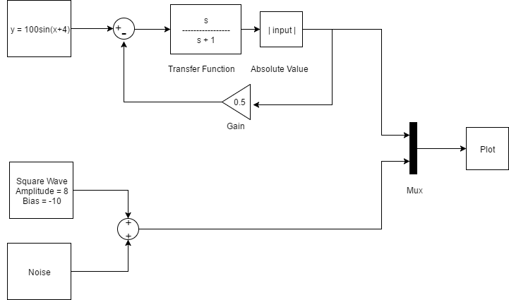
This example uses multiple input signals, a feedback loop, and a number of math elements. The resulting waves are muxed together so that they can both be output to the same plot.

In the equivalent qdex module, the simulation is started when the user presses the button, and stops after 10 seconds. Note that to output both waves to the same plot, the series attribute in the timePlot declaration must be set to 2.

sim-mux-transfer-function.jpg
<sectionNoTitle name="example2Section">

  <timePlot name="thisPlot" series="2" />

  <button content="Start Simulation">
    <onClick>
      anotherSim:Start()
    </onClick>
  </button>

  <simulation name="anotherSim" duration="10">
    <solver>
      <series>
        <mux>
          <series>
            <sine amplitude="100" phase="4" />
            <feedback>
              <series>
                <transferFunction num="1" den="1 1" />
                <math op="abs" />
              </series>
              <gain value="0.5" />
            </feedback>
          </series>
          <sum>
            <square amplitude="8" bias="-10" />
            <signalGenerator waveform="random" />
          </sum>
        </mux>
        <probe ref="example2Section.thisPlot" />
      </series>
    </solver>
  </simulation>

</sectionNoTitle>

Example 3

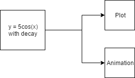
This is an example of a simple system being used to animate a shape. The source is created using a sine wave multiplied with a function in a system to create decay. Two plots inside a stack are used to plot the response and animate a ball.

sim-plot-animation.jpg
<include src="plotTools.xml" />

<section name="animationSection">
  <title>Bouncy Ball</title>

  <stack name="plotStack" orientation="horizontal">
    <timePlot name="responsePlot">
      <axis dim="x" min="0" max="5" />
    </timePlot>
    <xyPlot name="ballPlot">
      <axis dim="x" auto="growAndShrink" major="false" />
      <axis dim="y" auto="lockAspectRatio" major="false" />
      <series name="path" draw="lineSegments" />
      <series name="ball" draw="radialFill" />
      <!-- Transparent frame used to steady the plot as the ball moves -->
      <series name="frame">
        <style>
          <foreground color="transparent" />
        </style>
        <data>-1 6; 6 6; 6 -1; -1 -1</data>
      </series>
    </xyPlot>
  </stack>
  
  <!-- Drawing the ball -->
  <script>
    plotTools.drawCircle(plotStack.ballPlot.ball, {0,5}, 0.1)
  </script>

  <button content="Start">
    <onClick>
      ballSimulation:Start()
    </onClick>
  </button>

  <simulation name="ballSimulation" duration="5" period="0.005">
    <solver>
      <series>
        <sine amplitude="5" phase="1.57" />
        <system>
          <input name="sineIn" width="1" />
          <output name="decaySine" width="1" />
          <onOutputs>
            -- Creating decay
            return vector({sineIn[1]*(1/(0.75*time+1))})
          </onOutputs>
        </system>
        <math op="abs" /> <!-- Faking the presence of the ground, making ball "bounce" -->
        <probe ref="animationSection.plotStack.responsePlot" />
        <probe ref="animationSection.plotStack.ballPlot.path" />
        <system name="drawBall">
          <input name="ballLocation" width="1" />
          <onOutputs>
            -- Translating the ball using the value of the response 
            plotStack.ballPlot.ball.Transform = matrixf.translation(time, ballLocation[1]-5, 0)
          </onOutputs>
        </system>
      </series>
    </solver>
  </simulation>

</section>